



FastSlipPy is a scientific software package for modeling dynamic fault slip in induced seismicity. It is designed to simulate the behavior of faults under various stress conditions, providing insights into the mechanisms driving induced earthquakes. The software is based on the Finite Difference Method (FDM).
The initial version of this software is based on the open-source code IndNuc, which is a Matlab-based code specifically developed for modeling induced seismicity in Groningen area. FastSlipPy has been rewritten in Python to enhance its accessibility and usability, allowing for easier integration with other scientific tools and libraries.
The ambitious goal of FastSlipPy is to provide an easy-to-use, efficient, and flexible platform for the multi-scale and multi-physics modeling of induced seismicity, which may include the following features in the future:
- Multiscale modeling: coupling with Discrete Element Method (DEM) for the simulation of fault gouge.
- Multiphysics modeling: supporting the coupling of fluid, thermal, and mechanical processes.
- Main Features
- Dependencies
- Instructions
- Examples
- Documentation
- How to Contribute
- How to Cite
- Authorship
- License
This program can be used for modeling induced seismicity in a fault system. The main features of this program include:
- Easy-to-install and run on different platforms (Windows or Linux).
- Adaptive time stepping for efficient simulation of dynamic fault slip.
- Support different friction models, such as rate-and-state friction and others (under development).
- Support different fault angles.
- Post-processing in the format of both Paraview and Matplotlib for visualization of results.
- Modular design for easy integration with other scientific tools and libraries.
FastSlipPy is fully written in the Python programming language and adopts the Object Oriented Programming (OOP) paradigm to offer modularity and extensibility.
Please make sure you have installed Python3.X.X on your PC. Currently, Python3.10.X is recommended, as other versions haven't been tested.
All the required Python libraries will be added automatically. Some of them are:
- numpy
- matplotlib
- meshio
pip install fastslippy
Step 1: Download this software or use Git:
git clone https://github.com/ChengshunShang1996/FastSlipPy.git
Step 2: Installation.
(Windows users can jump this step) For Linux users, the virtual environment is suggested to be used:
python3 -m venv ~/my_env
source ~/my_env/bin/activate
In the project folder, run cmd command:
pip install -e .
Test it:
from fastslippy import FastSlipPy
For Linux or HPC users:
python3 -c "from fastslippy import FastSlipPy; print('Success')"
If you see the logo of FastSlipPy, you have successfully installed it. To run an example, please check the examples section.
- Input Parameters:
All the default parameters are defined in the file model_parameters.py. You can modify the parameters in the running script.
Grid stretching options are also available in model_parameters.py:
x_stretch_enabled,y_stretch_enabledx_stretch_inner_size,y_stretch_inner_sizex_stretch_inner_points,y_stretch_inner_pointsx_stretch_power,y_stretch_powerx_stretch_max_cell_size,y_stretch_max_cell_size(optional caps for the largest stretched cells)
If a max-cell-size cap is violated, FastSlipPy raises a ValueError and reports a suggested larger odd Nx/Ny while keeping the inner mesh point count unchanged.
By default, FastSlipPy uses a uniform grid.
Stretched mesh support in the elastic solver is currently experimental. To run with stretched mesh anyway, set:
allow_nonuniform_solver=True
If stretched mesh is enabled without this explicit opt-in, FastSlipPy now raises an error to prevent silently unreliable results.
Fault endpoint ownership is configurable independently of the named benchmark
with fault_reaches_surface and fault_reaches_bottom. Leaving either value as
None preserves the established defaults: both endpoints belong to the fault
for the California/BP3 case and to the outer boundary for the Lab and Groningen
cases. Traction-free and fault-interface stress operators themselves are shared
by all cases on both uniform and stretched meshes.
For large-scale runs that hit memory limits during sparse LU factorization, you can switch to the iterative linear solver in model_parameters.py:
linear_solver="iterative"iterative_method="gmres"(or"bicgstab")ilu_drop_tol,ilu_fill_factor,iterative_rtol,iterative_maxiter
By default, linear_solver="direct" is kept for backward compatibility. If direct LU runs out of memory, FastSlipPy can automatically fall back to iterative mode with:
fallback_to_iterative_on_oom=True
- Output files:
The output files are generated in the specified output directory [output] and
can be visualized using ParaView or Matplotlib. Matplotlib visualization is used
by default. Enable ParaView output with output_vtk_option=True; set
vtk_interval to control its cadence independently of checkpoints. The final
accepted state is always written when VTK output is enabled, and
vtu_results/results.pvd records the physical time of every frame.
Open that PVD file in ParaView to load the left domain, right domain, and fault
as one time-aware collection. Domain displacement, velocity, and quasi-static
shear stress are point data; quasi-static normal stress is quad cell data.
To run a simulation, use one of the short, self-contained scripts in the examples folder. For example:
python examples/run_case_groningen.py
or with your preferred way to run Python scripts. The simulation will start, and the output files will be generated in the specified output directory.
The examples folder contains the supported quick-start cases for Groningen,
laboratory shear, BP3, stretched meshes, and iterative solving. BP3 development
diagnostics, convergence studies, and plotting runners live under
tools/bp3/.
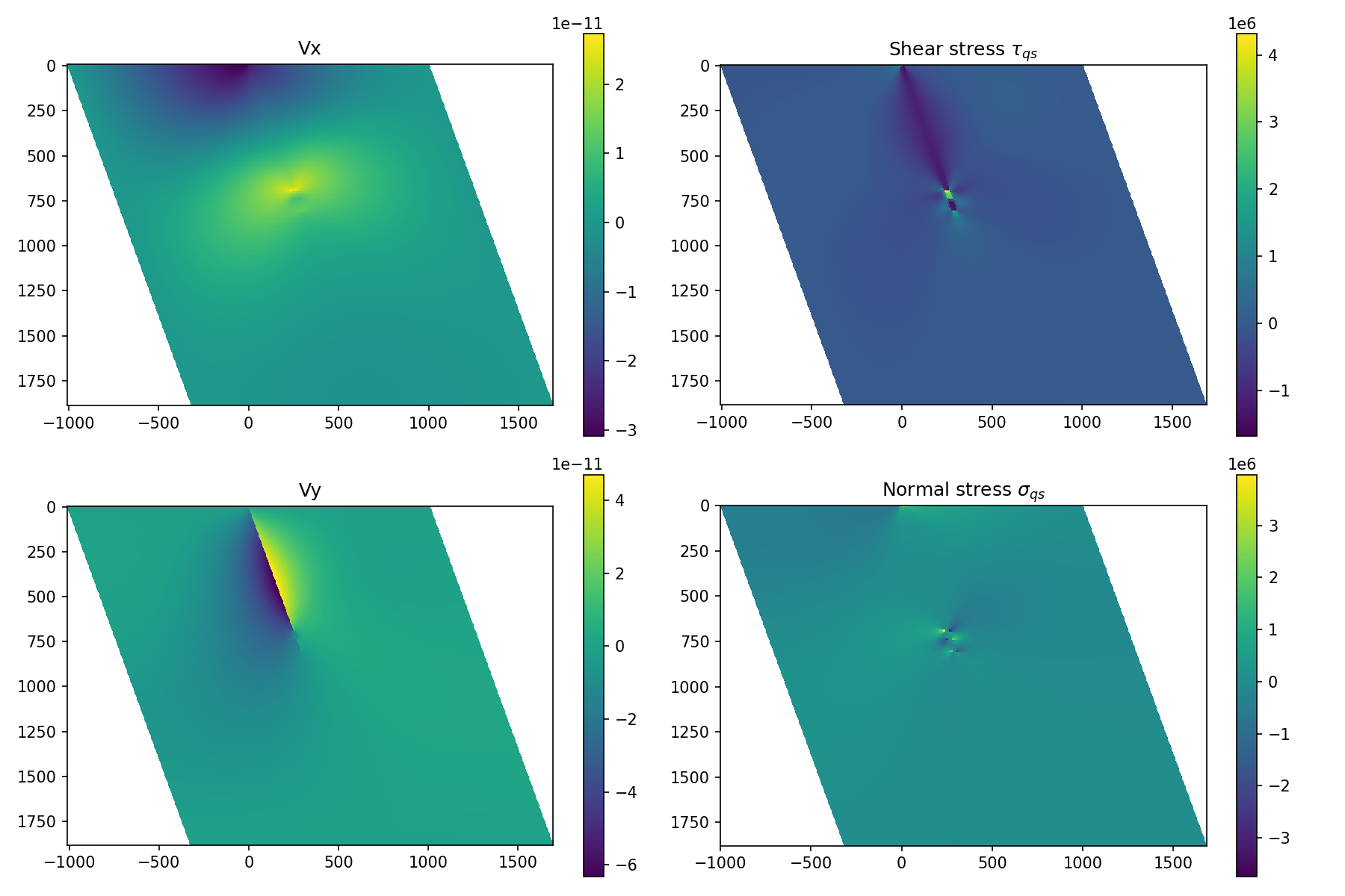
- Groningen case
- Lab-scale shear case
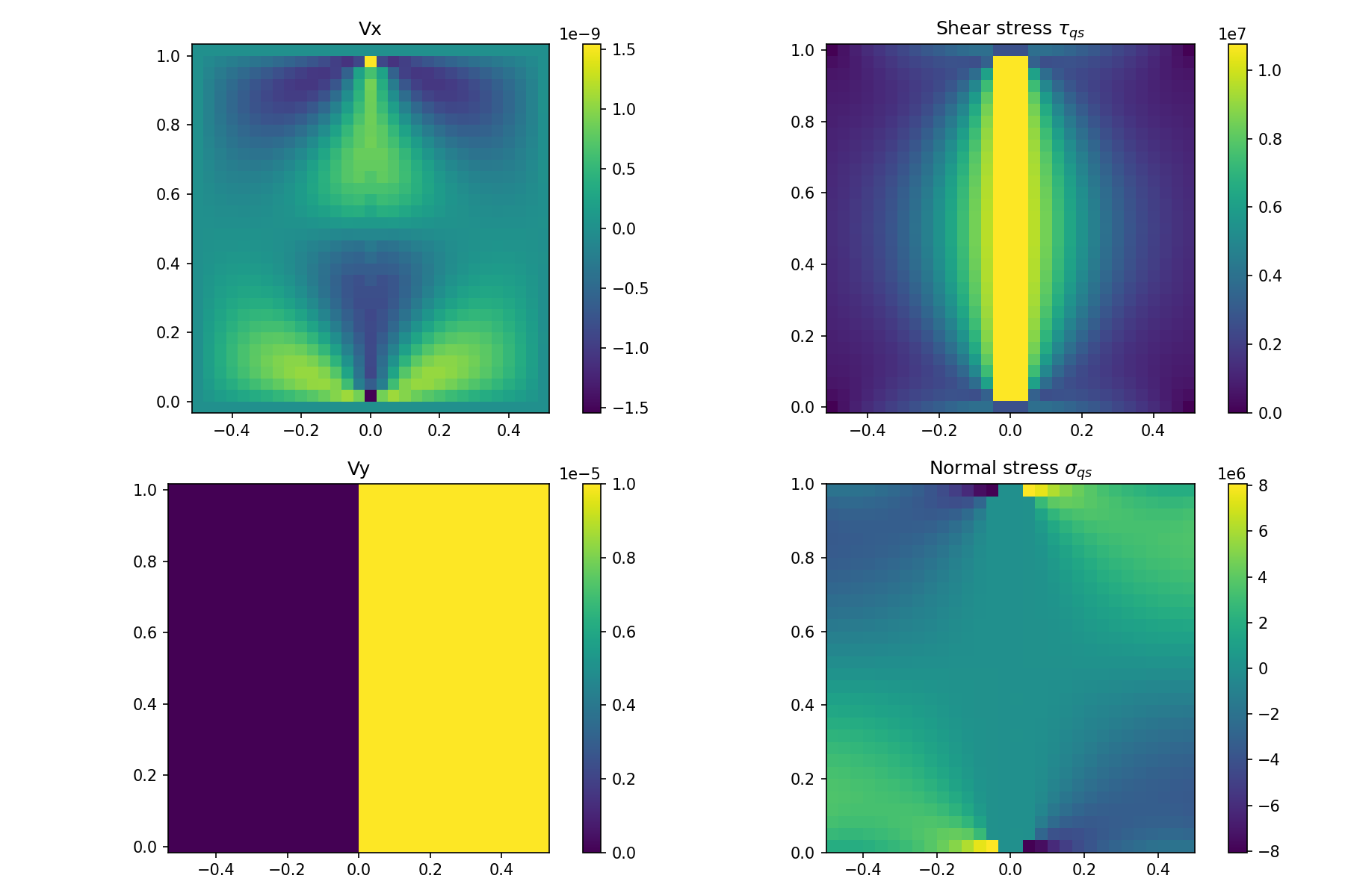
A high Young's modulus is used in the lab-scale shear case to generate the above figure.
Please read this README.md for information.
Use the same model configuration and output directory to resume a checkpoint:
model = FastSlipPy(params=params, output_dir="output", checkpointer=1000)
model.run()
This reads output/data_1000.npz. params.Nt specifies additional steps;
params.tfinal remains the absolute end time. Output and checkpoint intervals
use cumulative step numbers, including VTK filenames.
On restart, dataall.npz retains samples through the checkpoint time and
appends new samples. Samples after an earlier restart point are replaced.
BP3 surface histories and exported station files follow the same history.
Only written samples are saved, without unused zero-filled columns. Keep
dataall.npz alongside the checkpoint: missing or previously overwritten
history cannot be reconstructed from a single checkpoint. Older histories
without surface data retain missing surface samples as NaN.
Restarting at or beyond tfinal leaves existing result files untouched.
Groningen checkpoints now include both pore-pressure fields; older checkpoints
reconstruct them from elapsed time and the configured loading schedule.
Please check the contribution guidelines.
To cite this repository, you can use the metadata from this file.
- Chengshun Shang 1 (c.shang@uu.nl)
1 Utrecht University (UU)

The program was initially developed under the context of the FastSlip project. The author would like to thank the project team (Dr. André Niemeijer et al.) for their support and guidance. The author also acknowledges the contributions of the open-source community, particularly the developer of IndNuc, Dr. Meng Li, whose work served as a foundation for this software.
FastSlipPy is licensed under the MIT license, which allows the program to be freely used by anyone for modification, private use, commercial use, and distribution, only requiring the preservation of copyright and license notices. No liability and warranty are provided.