


Detect marine heatwaves (MHW), marine cold spells (MCS) and atmospheric heatwaves (AHW) on the grid you already have, then follow them as connected objects that split and merge through time.
xHW is a Python library built on NumPy, xarray and SciPy. It turns daily temperature into a fitted reference and threshold, a per-cell event mask, an event catalog, daily spatial patches, optional overlap tracking and a genealogy of branches and spacetime events. Each product keeps its own evidence: an exceedance, a day joined across a short gap, and a cell added by spatial processing are stored separately and never confused.
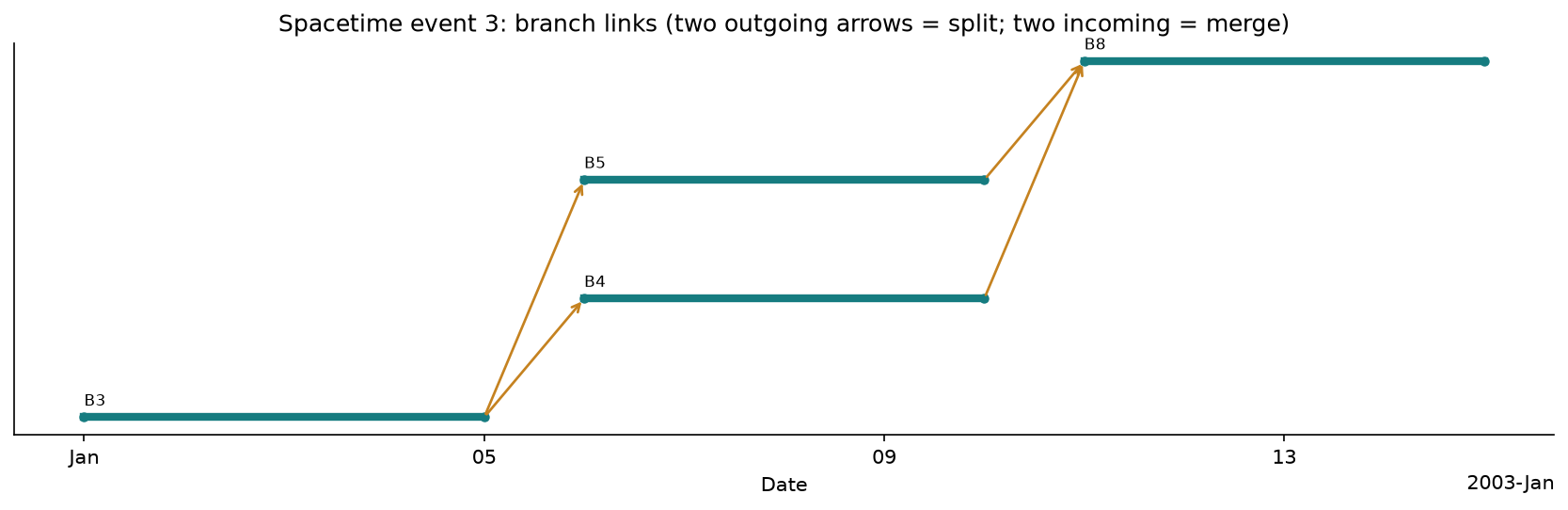
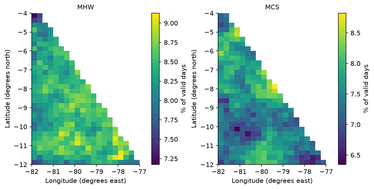
Top: executed synthetic example. One patch splits on day 6 and merges on day 11, giving four branches and one 15-day spacetime event. Arrows mean overlap, not causation. Bottom: percentage of valid days inside MHW (P90) and MCS (P10) events in a seeded synthetic reconstruction of the SST field off Peru, 1991–2025, generated in a second; it is not an observation. Both figures come from the tutorials.
- Three phenomena, one model. MHW and MCS (Hobday et al. 2016 thresholds and persistence) and AHW (TX90, TN90 and a joint daily TX+TN profile).
- Seven baselines. A fixed seasonal climatology and six dynamic references: detrended, shifting, STL, state space, GAM and SSA. All can be fitted retrospectively or causally, with optional within-reference correction.
- Native grids. Points, lines, surfaces and volumes on structured or curvilinear grids, with physical cell measures (m, m², m³). No regridding is required.
- Explicit evidence.
exceedance,event_membership,joined_gap,validand bit-codedinvalid_reasonare separate layers. Missing data is never read as "no event". - Objects, tracking and genealogy. Ordered spatial recipes (morphology, connectivity, area filters), overlap tracking, and a lineage graph that keeps every parent and child.
- Weighted metrics. Area- or volume-weighted size, size-time, footprint, displacement and signed intensity, for each branch and spacetime event.
- Reproducible. Every spec is an immutable, serializable dataclass, and the test suite (about 800 tests) and every tutorial here run offline. Real-data cases, with checksums, live in xhw-benchmark.
Python 3.11 or newer. From a source checkout:
python -m venv .venv
source .venv/bin/activate          # Windows PowerShell: .venv\Scripts\Activate.ps1
python -m pip install .
python examples/quickstart.py # prints "xHW 0.0.1: known 10-day synthetic event detected"| Extra | Adds | Needed for |
|---|---|---|
| (core) | NumPy, xarray, SciPy | Everything below, including the vectorized STL, GAM and SSA engines |
.[dynamic] |
statsmodels, pygam | state_space baselines and the statsmodels/pygam reference engines |
.[parallel] |
Dask | Lazy temporal operations on chunked data |
.[dev] |
pytest, Ruff, numerical test engines, Matplotlib, Plotly and widgets | Complete test suite |
examples/requirements-interactive.txt |
Plotly, ipywidgets, Pillow and example tools | GIF and interactive examples |
examples/requirements.txt |
Matplotlib, h5netcdf, Jupyter | Tutorials, notebooks and figures |
From this source checkout, use the deterministic tutorial's ready temperature, grid,
baseline specification and event definition. Here mhw is an ordinary Python alias:
import sys
sys.path.insert(0, "examples")
from _data import synthetic_inputs
import xhw

ds, grid, baseline, mhw = synthetic_inputs()
fitted = xhw.fit_baseline(ds, variable="sst", grid=grid, baseline=baseline, definition=mhw)
mask = xhw.detect(ds, variable="sst", grid=grid, definition=mhw, baseline_result=fitted)
mask.check_invariants()
If a compatible fitted baseline is already prepared, only the final detect call is needed.
mhw.to_dict() and baseline.to_dict() expose the scientific choices. The examples'
profiles.example_profiles() also returns MCS, TX90, TN90 and TX+TN configurations;
these are not new defaults of the installed API. The complete standalone example follows.
The block below runs as is. It builds 34 years of daily SST on an 8 × 8 grid and
injects a warm patch in June 2015 whose middle row cools for a week, so the patch
splits in two and merges again. To use your own data, replace the
first block with ds = xr.open_dataset("my_sst.nc") plus a domain_mask and a
cell_area variable.
import numpy as np
import xarray as xr

import xhw

# --- 1. Daily temperature on a small surface grid --------------------------------------
time = np.arange(np.datetime64("1982-01-01"), np.datetime64("2016-01-01"))
lat, lon = np.arange(-12.0, -4.0), np.arange(-82.0, -74.0)
day_of_year = (time - time.astype("datetime64[Y]")).astype(int)
season = 20 + 3 * np.sin(2 * np.pi * day_of_year / 365.25)
rng = np.random.default_rng(0)
sst = season[:, None, None] + rng.normal(0, 0.5, (time.size, lat.size, lon.size))
start = int(np.flatnonzero(time == np.datetime64("2015-06-01"))[0])
sst[start:start + 20, 2:5, 2:7] += 4.0       # a 3 x 5 warm patch for 20 days ...
sst[start + 7:start + 14, 3, 2:7] -= 4.0     # ... whose middle row cools for a week

area = (6_371_000.0**2 * np.deg2rad(1.0)
        * np.abs(np.sin(np.deg2rad(lat + 0.5)) - np.sin(np.deg2rad(lat - 0.5))))
ds = xr.Dataset(
    {"sst": (("time", "lat", "lon"), sst, {"units": "degC"}),
     "domain_mask": (("lat", "lon"), np.ones((lat.size, lon.size), bool)),
     "cell_area": (("lat", "lon"), np.repeat(area[:, None], lon.size, 1), {"units": "m2"})},
    coords={"time": time.astype("datetime64[ns]"), "lat": lat, "lon": lon},
)

# --- 2. Declare the grid, the data source and the scientific choices ------------------
grid = xhw.GridSpec(
    support="surface", topology="structured", time_dim="time", spatial_dims=("lat", "lon"),
    coords=xhw.CoordRoles(lat="lat", lon="lon"), calendar="standard", frequency="1D",
    time_axes="single", periodic_x=False,
    cell_measure=xhw.CellMeasure(kind="area", var="cell_area", units="m2"),
    vertical=None, domain="ocean", domain_mask="domain_mask", domain_fraction=None,
    native=xhw.NativeGrid(product="synthetic", resolution="1 degree", is_native=True))
grid.check(ds)

source = xhw.SourceRef(dataset_id="synthetic:readme", variable="sst",
                       accessed="2026-10-11", product_status="final")
baseline = xhw.BaselineSpec(               # Hobday et al. (2016) fixed climatology
    method="fixed_climatology", computed_on="temperature",
    reference_period=("1983-01-01", "2012-12-31"), source=source,
    doy_window_days=11, smoothing_window_days=31, percentile_estimator="hyndman_fan_7",
    leap_day_policy="hobday_366_interp", min_samples=264,
    fit_mode="retrospective", available_until=None)
definition = xhw.DefinitionSpec(           # MHW: > P90 for >= 5 days, gaps <= 2 days joined
    profile="hobday2016", phenomenon="mhw", variable="sea_surface_temperature",
    combination="single", daily_statistic="native", day_definition="native",
    tail="upper", comparator=">", threshold_kind="percentile", percentile=90.0,
    absolute_threshold=None, min_duration_days=5, max_gap_days=2,
    join_rule="qualify_then_join", missing_policy="as_non_exceedance",
    season_months=None, category_scheme="hobday2018")

# --- 3. Baseline and threshold -> detection -> per-cell event catalog ----------------
fitted = xhw.fit_baseline(ds, variable="sst", grid=grid, baseline=baseline,
                          definition=definition)
mask = xhw.detect(ds, variable="sst", grid=grid, definition=definition,
                  baseline_result=fitted)
catalog = xhw.build_catalog(mask, analysis_mode="retrospective")

# --- 4. Daily patches -> overlap tracking -> genealogy --------------------------------
recipe = xhw.SpatialRecipe(input_layer="event_membership", steps=(
    xhw.RecipeStep.segment(footprint=xhw.Footprint.connected(1),
                           min_area=xhw.MinArea.none()),
    xhw.RecipeStep.track(min_overlap=0.1, max_gap_days=0, min_duration_days=5),
))
objects = xhw.build_objects(mask, recipe=recipe)
graph = xhw.build_lineage(objects, field=mask.intensity(), weighted=True)

largest = int(np.argmax(graph.dataset.event_area_days.values))     # by area x days
event = int(graph.dataset.event_number.values[largest])
series = graph.series(spacetime_event=event)         # daily area, intensity, ...
print(catalog.dataset.sizes["event"], "per-cell events;",
      graph.dataset.sizes["spacetime_event"], "spacetime events;",
      f"largest lasts {int(graph.dataset.event_duration_days.max())} days")
Plot the products with xarray and Matplotlib. xHW has no plotting API of its own; the plotting guide collects ready-made recipes.
import matplotlib.pyplot as plt

fig, (left, right) = plt.subplots(1, 2, figsize=(10, 3.5), layout="constrained")
valid_days = mask.dataset.valid.sum("time")
frequency = 100 * (mask.dataset.event_membership & mask.dataset.valid).sum("time")
(frequency / valid_days.where(valid_days > 0)).plot(ax=left, cbar_kwargs={"label": "% of valid days"})
left.set_title("MHW frequency")
(series.area / 1e6).plot(ax=right)
right.set(title=f"Spacetime event {event}", ylabel="Occupied area (km²)")
plt.show() daily temperature (xarray)
│ aggregate_daily() hourly → daily, with sample counts (optional)
│ interpolate_gaps() short interior gaps, flagged "filled" (optional)
▼
1. BASELINE fit_baseline() ──► BaselineResult reference + threshold
▼
2. DETECT detect() ──► XMask exceedance, membership, validity
├──────────────► build_catalog() ──► EventCatalog one row per event and cell
▼
3. OBJECTS build_objects() ──► ObjectField daily patches (+ track IDs if asked)
▼
4. GENEALOGY build_lineage() ──► LineageGraph branches, splits, merges, events
▼
5. ANALYSE graph.series() / graph.maps() / xarray + Matplotlib (examples/plotting.py)
You can stop at any stage: a temporal study ends at the catalog, and a spatial study
can skip tracking because build_lineage also works on untracked patches.
| Stage | Function | Input → output | Main choices |
|---|---|---|---|
| Prepare | aggregate_daily, interpolate_gaps, GridSpec.check |
Raw samples → regular daily dataset | Units, calendar, day clock, statistic, gap length |
| Baseline | fit_baseline |
Daily temperature + BaselineSpec → BaselineResult |
Method, reference period, window, estimator, leap days |
| Detect | detect |
Temperature + baseline + DefinitionSpec → XMask |
Tail, percentile, minimum duration, gaps, missing policy |
| Catalog | build_catalog |
XMask → EventCatalog |
Retrospective or monitoring mode, censoring |
| Objects | build_objects |
XMask + SpatialRecipe → ObjectField |
Input layer, connectivity, area filter, morphology, order |
| Tracking | RecipeStep.track |
Daily patches → track IDs | Overlap measure and threshold, object gaps, duration |
| Genealogy | build_lineage |
ObjectField → LineageGraph |
LinkPolicy, merge rule, intensity weighting |
Details: processing guide.
These snippets continue the quick-start session.
fit_baseline returns a BaselineResult, not events. The fixed climatology pools an
11-day window around each day of the year over the reference period, takes the
90th percentile, and smooths it with a 31-day moving average:
clim = fitted.dataset
print(clim.reference.dims)                  # ('dayofyear', 'lat', 'lon') for a fixed baseline
print(float(clim.threshold.isel(dayofyear=180, lat=3, lon=3)), "degC on day 181")
fitted.check_invariants()
Dynamic baselines model a trend and a seasonal cycle, then add a percentile of the residual:
temperature = trend + seasonal + residual
reference(t) = trend(t) + seasonal(t)
threshold(t) = reference(t) + percentile_p(residual | day of year)
from dataclasses import replace

detrended = replace(baseline, method="detrended",
                    params=(("trend_degree", 1), ("n_harmonics", 3)))
fitted_dynamic = xhw.fit_baseline(ds, variable="sst", grid=grid,
                                  baseline=detrended, definition=definition)
print(fitted_dynamic.dataset.threshold.dims)   # ('time', 'lat', 'lon'): varies in time
See Baseline types for the seven methods and their engines.
detect compares each valid day with its threshold, keeps runs of at least
min_duration_days, and joins runs separated by up to max_gap_days. The result is
an XMask whose layers stay separate:
| Variable | Meaning |
|---|---|
exceedance |
The temperature is beyond the threshold on that day |
event_membership |
The day belongs to a qualifying event, including joined gap days |
joined_gap |
Membership without exceedance (a short cool or missing day inside an event) |
valid |
Temperature, baseline and data quality allow interpretation |
invalid_reason |
Bit flags: 1 outside domain, 2 missing, 4 undefined baseline, 8 few samples, 16 low quality |
cell = mask.dataset.isel(lat=3, lon=3).sel(time=slice("2015-06-01", "2015-06-25"))
print({name: int(cell[name].sum()) for name in ("exceedance", "event_membership", "joined_gap")})
intensity = mask.intensity() # temperature − reference, signedtable = catalog.dataset[["start", "end", "duration_days", "intensity_max", "category_max"]]
print(table.sortby("duration_days", ascending=False).isel(event=slice(0, 3)))
catalog.check_against(mask)One row per event and cell: counting rows is not the same as counting distinct spatial heatwaves. That is what the object and genealogy stages do.
The default recipe (SpatialRecipe.default()) segments exceedances into face-connected
patches of at least 5% of the domain, then applies persistence. It does not track.
Tracking is an explicit last step, linking patches that share grid cells on consecutive days:
print(objects.dataset[["object_time", "object_area", "object_cells"]].to_dataframe().head())
print(graph.dataset.sizes["branch"], "branches;",
      int(graph.dataset.is_split.sum()), "splits;", int(graph.dataset.is_merge.sum()), "merges")
edges = graph.transitions()                 # every candidate link, with its overlap measures
maps = graph.maps(objects, spacetime_event=event)    # footprint and occupied days per cell
A branch is a chain of one-to-one links; a split or merge ends a branch and starts new ones. A spacetime event is a connected group of linked patches. See objects and genealogy and metrics.
DefinitionSpec.phenomenon selects what is detected. The other fields state the rule
explicitly, because a profile name alone does not fill in scientific choices.
| Phenomenon | Typical definition | tail / comparator |
Daily input | Categories |
|---|---|---|---|---|
| MHW: marine heatwave | SST > P90, ≥ 5 days, gaps ≤ 2 days | upper / > |
Native daily SST | hobday2018 (moderate to extreme) |
| MCS: marine cold spell | SST < P10, ≥ 5 days, gaps ≤ 2 days | lower / < |
Native daily SST | schlegel2021 |
| AHW: atmospheric heatwave, TX90 | TX > P90, ≥ 3 days | upper / > |
Daily max (daily_statistic="max") |
none |
| AHW: TN90 | TN > P90, ≥ 3 days | upper / > |
Daily min (daily_statistic="min") |
none |
| AHW: joint TX+TN | TX and TN both > P90 on the same day (or TN lagged), ≥ 3 days | upper / > |
Two components, combination="and_daily" |
none |
The threshold can be a percentile (threshold_kind="percentile") or a fixed value
(threshold_kind="absolute", for example (28.0, "degC")). season_months restricts
detection to some months.
mcs = replace(definition, profile="schlegel2021", phenomenon="mcs", tail="lower",
              comparator="<", percentile=10.0, category_scheme="schlegel2021")
above_28 = replace(definition, profile="absolute_28C", threshold_kind="absolute",
                   percentile=None, absolute_threshold=(28.0, "degC"), category_scheme=None)

ahw_common = dict(phenomenon="ahw", day_definition="offset:-05:00", tail="upper",
                  comparator=">", threshold_kind="percentile", absolute_threshold=None,
                  min_duration_days=3, max_gap_days=0, join_rule="qualify_then_join",
                  missing_policy="as_non_exceedance", season_months=None,
                  category_scheme=None)
tx90 = xhw.DefinitionSpec(profile="perkins2013_tx90", variable="tx_daily",
                          combination="single", daily_statistic="max", percentile=90.0,
                          **ahw_common)
tx_and_tn90 = xhw.DefinitionSpec(
    profile="xhw_txtn90", variable="tx_daily&tn_daily", combination="and_daily",
    daily_statistic="native", percentile=None,
    components=(xhw.DailyComponent(variable="tx_daily", daily_statistic="max",
                                   percentile=90.0, lag_days=0),
                xhw.DailyComponent(variable="tn_daily", daily_statistic="min",
                                   percentile=90.0, lag_days=0)),
    **ahw_common)
For AHW, hourly data is first reduced to local days with aggregate_daily. It records
which clock the timestamps use and how many samples each day had. The
ERA5 tutorial in xhw-benchmark runs all four AHW
profiles over land and ocean air.
BaselineSpec.method selects the reference. Method parameters go in the params tuple.
Unknown parameters raise ValidationError when fitting.
method |
What it models | Default parameters (0.0.1) | Engines |
|---|---|---|---|
fixed_climatology |
Day-of-year percentile over a fixed reference period (Hobday et al. 2016) | Window and smoothing from the spec | core |
detrended |
Polynomial trend + annual harmonics (or a climatology of the detrended series) | trend_degree=1, n_harmonics=3, seasonal="harmonic" |
core |
shifting |
Seasonal mean over the preceding years | window_years=30, min_years=10 |
core |
stl |
Seasonal-trend decomposition by LOESS (Cleveland et al. 1990) | trend_window_days=7305, seasonal_window="periodic", robust=0 |
engine="vectorized" (default) or "statsmodels" (needed for robust=1; cell by cell, slow) |
state_space |
Local linear trend + trigonometric seasonality (Kalman smoother) | n_harmonics=3, trend_timescale_days=5600 |
statsmodels (.[dynamic]) |
gam |
Penalized spline trend + cyclic seasonal spline | trend_splines_per_decade=1.5, seasonal_splines=20, trend_lam=seasonal_lam=0.6 |
engine="vectorized" (default) or "pygam" |
ssa |
Singular spectrum analysis: low-frequency components form the trend | window_days=5479, n_components=12, trend_period_days=10958 |
core |
Choices that apply to every method:
| Field | Options | Meaning |
|---|---|---|
fit_mode |
retrospective, causal |
Causal fitting uses only data available by available_until (causal_scheme="cutoff" or "expanding") |
in_base_correction |
none, leave_one_year_out, mean_threshold |
Stops reference years from being judged against a threshold they helped estimate (Zhang et al. 2005); in_base_rates gives bootstrap rates |
percentile_estimator |
hyndman_fan_1 … hyndman_fan_9 |
Explicit sample-quantile definition (Hyndman & Fan 1996) |
leap_day_policy |
hobday_366_interp, calendar_doy, not_applicable |
How February 29 enters the day-of-year climatology |
robust_stl = replace(baseline, method="stl",
                     params=(("engine", "statsmodels"), ("robust", 1)))
causal = replace(detrended, fit_mode="causal", available_until="2012-12-31",
                 params=(("causal_scheme", "cutoff"), ("max_extrapolation_days", 30)))
corrected = replace(baseline, in_base_correction="leave_one_year_out")
These defaults reproduce the validated configurations; they are not universally optimal. The baseline guide covers memory cost, causal limits and the measured differences between engines.
| Step | Options |
|---|---|
| Input layer | exceedance (daily evidence) or event_membership (after temporal persistence) |
| Connectivity | Footprint.connected(rank): rank 1 = faces (4 on surfaces, 6 in volumes), rank 2/3 add edges and corners; Footprint.disc(radius_km); Footprint.explicit(offsets); vertical_gap_m for physical vertical links |
| Morphology | RecipeStep.morph("open" or "close", footprint); changed cells are kept in added/removed |
| Area filter | MinArea.default() (5% of the domain), none(), percentile, absolute_km/km2/km3 |
| Persistence | RecipeStep.persist(...) per cell on the processed geometry |
| Tracking | RecipeStep.track(min_overlap, max_gap_days, min_duration_days, link_measure=...); link_measure is overlap_smaller, iou, source_fraction or target_fraction; analysis_mode is retrospective or monitoring |
| Genealogy | LinkPolicy(measure, threshold, max_gap_days); merge_rule is new_event or survivor |
| Other tools | partition_merges, ingest_objects / compare_objects (external labels), neighbor_fraction |
xHW analyses files you open with xarray; it never downloads data. Everything in this repository runs offline on synthetic data, in minutes: the tutorials generate their input and the tests need no files. The real cases live in a companion project, xhw-benchmark:
| Case | Data | What it shows |
|---|---|---|
| OISST Peru | NOAA OISST v2.1, 0.25° | MHW/MCS, fixed versus detrended baseline, objects, genealogy |
| OSTIA versus OISST | Met Office OSTIA at 0.05° and 0.25°, and OISST | Product and resolution effects, in three arms |
| OISST equatorial Pacific | NOAA OISST, Niño 3.4 box (5°S–5°N, 170°W–120°W), 8 000 ocean cells | MHW/MCS and the 2015–16 El Niño as one large object, with its genealogy |
| ERA5 Peru | ERA5 TX/TN, local days | Hourly aggregation, TX90, TN90 and joint TX+TN over land and ocean air |
| GLORYS volume | GLORYS12V1 thetao |
Voxel detection, vertical connectivity, volumetric genealogy |
That project holds the compressed NetCDF datasets (about 300 MB, as release assets) with two hashes each, so a copy can be verified even after recompression; their downloaders; the processed products; and the notebooks. Your own data go through the same stages: see data and provenance.
| Tutorial | Shows | Notebook / script |
|---|---|---|
| Synthetic (no data) | Every stage on a hand-checkable field: gaps, morphology, connectivity, one split and one merge | notebook · script |
| Synthetic Peru (no data) | A seeded reconstruction of the OISST case off Peru: MHW and MCS, fixed versus detrended baselines, daily patches, tracking, genealogy | notebook · script |
| API walkthrough | Ingestion, comparison, partition, in-base rates, serialization | script |
The notebooks are saved with their outputs, so they can be read on GitHub. The real-data tutorials (OISST over Peru and the equatorial Pacific, OSTIA, ERA5, GLORYS) are in xhw-benchmark.
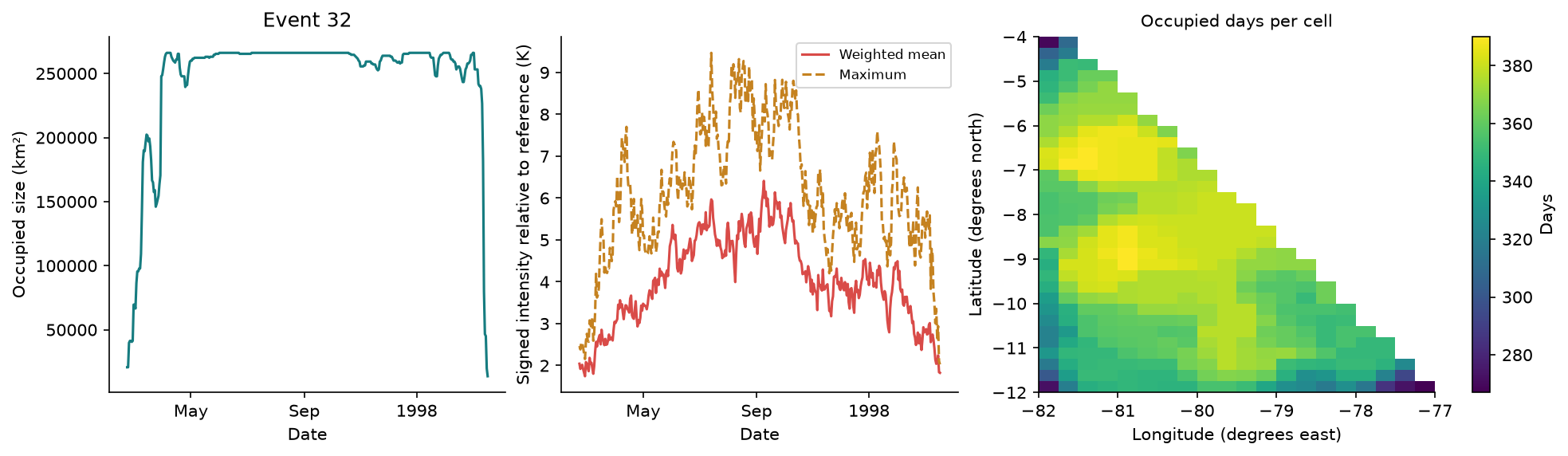
Largest spacetime event of the synthetic Peru field: occupied area, area-weighted intensity and occupied days per cell.
| Read | To |
|---|---|
| Getting started | Install and run a first detection |
| Processing guide | Follow each stage, its inputs, outputs and quality checks |
| Baselines | Choose and configure a reference and threshold |
| Objects and genealogy | Build patches, track them and read the lineage graph |
| Metrics · Plotting | Compute tables and draw figures |
| Data · Tutorials | Prepare your inputs and run the two synthetic tutorials |
| API reference | Look up all 44 public names |
| Scientific contract · Validation · Reproducibility | Check limits, evidence and recorded runs |
python -m pip install ".[dev]"
python -m pytest
python -m ruff check .
Tests run offline. They include analytical cases and stored comparisons with marineHeatWaves, climdex, R and statsmodels STL, ssalib, Ocetrac and marEx; none of those packages is needed to run them. Reproducing a result is not the same as a scientific review: each real example states its review status. See validation and capabilities and evidence.
Please cite the methods your configuration uses, for example:
- Hobday, A. J. et al. (2016). A hierarchical approach to defining marine heatwaves. Progress in Oceanography 141, 227–238. doi:10.1016/j.pocean.2015.12.014
- Hobday, A. J. et al. (2018). Categorizing and naming marine heatwaves. Oceanography 31(2), 162–173. doi:10.5670/oceanog.2018.205
- Perkins, S. E. and Alexander, L. V. (2013). On the measurement of heat waves. Journal of Climate 26, 4500–4517. doi:10.1175/JCLI-D-12-00383.1
Complete method references and verified identifiers, including Bonino STL attribution and Schlegel cold categories, are in the methodological bibliography. Software and data credit remain in sources and attribution.
Copyright 2026 Daniel Camarena. Licensed under Apache-2.0. Questions, bug reports and feature requests: GitHub issues.